9 Compose

The “Compose” tab is where you calculate the index scores, as well as any other aggregate scores. This effectively generates the results of the index, although there are further tabs for exploring the data and making adjustments later on.

9.1 About

Calculating index scores is done by mathematical aggregation of indicators. As discussed in Chapter 8, indicators must be normalised first so that they are on a common scale.

There are two simple aggregation methods available in the app. The first is the weighted arithmetic mean. Denoting a group of indicators as \(x_i \in \{x_1, x_2, ... , x_d \}\), the weighted arithmetic mean is calculated as:

\[ y = \frac{1}{\sum_{i=1}^d w_i} \sum_{i=1}^d x_iw_i \]

where the \(w_i\) are the weights corresponding to each \(x_i\). Here, if the weights are chosen to sum to 1, it will simplify to the weighted sum of the indicators. In any case, the weighted mean is scaled by the sum of the weights, so weights operate relative to each other.

Clearly, if the index has more than two levels, then there will be multiple aggregations. For example, there may be three groups of indicators which give three separate aggregate scores. These aggregate scores would then be fed back into the weighted arithmetic mean above to calculate the overall index.

The arithmetic mean has “perfect compensability”, which means that a high score in one indicator will perfectly compensate a low score in another. In a simple example with two indicators scaled between 0 and 10 and equal weighting, a unit with scores (0, 10) would be given the same score as a unit with scores (5, 5) – both have a score of 5.

An alternative is the weighted geometric mean, which uses the product of the indicators rather than the sum.

\[ y = \left( \prod_{i=1}^d x_i^{w_i} \right)^{1 / \sum_{i=1}^d w_i} \]

This is simply the product of each indicator to the power of its weight, all raised the the power of the inverse of the sum of the weights.

The geometric mean is less compensatory than the arithmetic mean – low values in one indicator only partially substitute high values in others. For this reason, the geometric mean may sometimes be preferred when indicators represent “essentials”. An example might be quality of life: a longer life expectancy perhaps should not compensate severe restrictions on personal freedoms.

Regardless of the aggregation method, the aggregation follows the structure of the index from the lowest level upwards. The indicators (at level 1) are first aggregated within their groups to give the aggregate scores at level 2. The aggregates at level 2 are then aggregated together within their groups to give the aggregates at level 3, and so on, up to the index level.

At the aggregation step it is also possible to build in data availability restrictions, which is available in the {composer} app. By default, for a given unit, an aggregate can be given a score as long as at least one data point is available - the aggregation methods above take the mean only over the available points. For example, consider the indicator values of two units and their aggregate scores:

Unit A has normalised indicator values Ind1 = 20, Ind2 = 35, Ind3 = 70, Ind4 = 18 and Ind5 = 12 for a given indicator group. The aggregate score is calculated as the equally weighted mean: 31.
Unit B has missing data for four out of the same five indicators, but has a value for Ind4, which is 65. The aggregate score is calculated as the mean of the available points, which gives 65.

Here, the second case can be quite misleading since the score is based on an indicator group with 80% missing data.

To avoid this, you can set a data availability limit which is applied individually to each aggregation. For example, setting the limit at 0.6 would mean that, for each unit and each aggregation, a score is only calculated if the unit has at least 60% data availability (in that aggregation group) - if the availability is lower, the score is treated as a missing value.

This safeguard is usually a sensible approach to avoid overstating what is actually known. Note that this is different from the overall unit screening described in Chapter 5, because it is applied to each aggregation group individually.

9.2 How

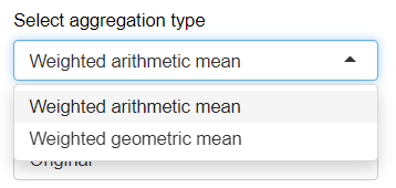
In the app, the aggregation methods mentioned above can be selected in the sidebar under the “aggregation type” dropdown.

Underneath this, there is the option to select the weight set to use in the aggregation. Weight sets are named sets of weights for all indicators and aggregates. The default, “Original”, is the set of weights specified in the “iMeta” table in your input data. Alternatively, the “Equal” weight set specifies equal weights everywhere.

Later, in Chapter 15, you will discover how to build alternative weight sets in the “Reweighting” tab of the app, which can be selected here. If you have not been to the Reweighting tab yet and built any weight sets, the only two options will be those mentioned above. See Chapter 15 for more details on weight sets.

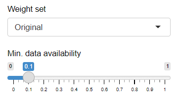
The final input is the data availability threshold which was discussed in the previous section. If you don’t want to impose any data availability threshold, simply set this to zero. Consider also that if you have imputed your data, you will probably have no missing data points, so the data availability threshold will have no effect.

Finally, click the “Run” button to generate the results. This will generate a summary table of the results, colour-formatted to help highlight high and low values. The table rows are sorted by the highest index score downwards, and the columns are sorted from the highest level downwards. You can sort the table by different columns by clicking on the column headers, and search for particular units using the search box.

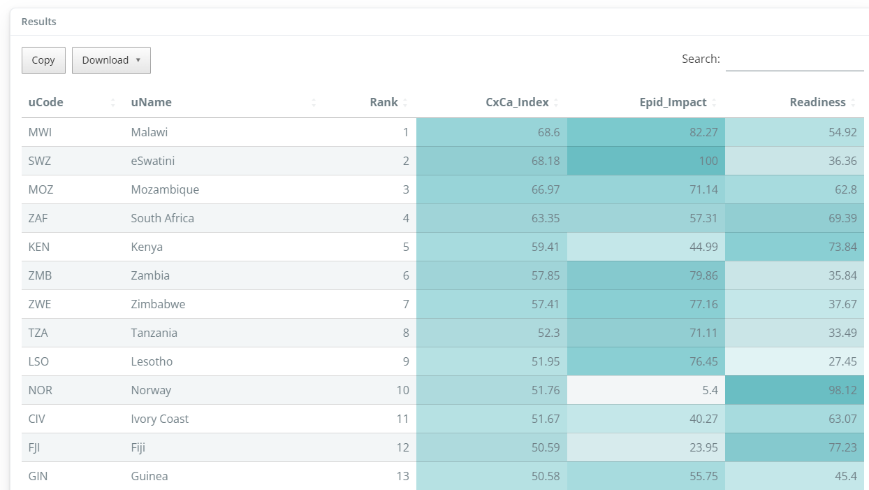
Keep in mind that it is up to you to interpret the results correctly: in some indexes, higher values may be “better”, in others they may be “worse”. This may be a good moment to look critically at the results and consider whether the index measures what it is you want to measure, and whether the directionality of each indicator, each dimension and the index itself is suitable. Moreover, you may wish to pass prelimary results to topical experts and stakeholders as a “reality check” - this may result in some feedback at this initial stage.