13 Correlations
Correlations measure the strength of relationships between variables.
The correlations tab allows you to understand relationships between indicators and aggregates by using heat maps. Correlations are very useful in analysing a data set, and can point to such things as:
- Indicators which are very similar and imply double-counting
- Indicators which run against the direction of other indicators and may not conceptually fit the framework
- Possible errors in assigning directions
In general, it is useful to focus on very high correlations or negative correlations, which point to the cases above.
13.1 App usage
To generate correlation plots use the sidebar options. By default, when clicking the “Run” button, all indicators should be correlated against all other indicators, resulting in a plot something like this:
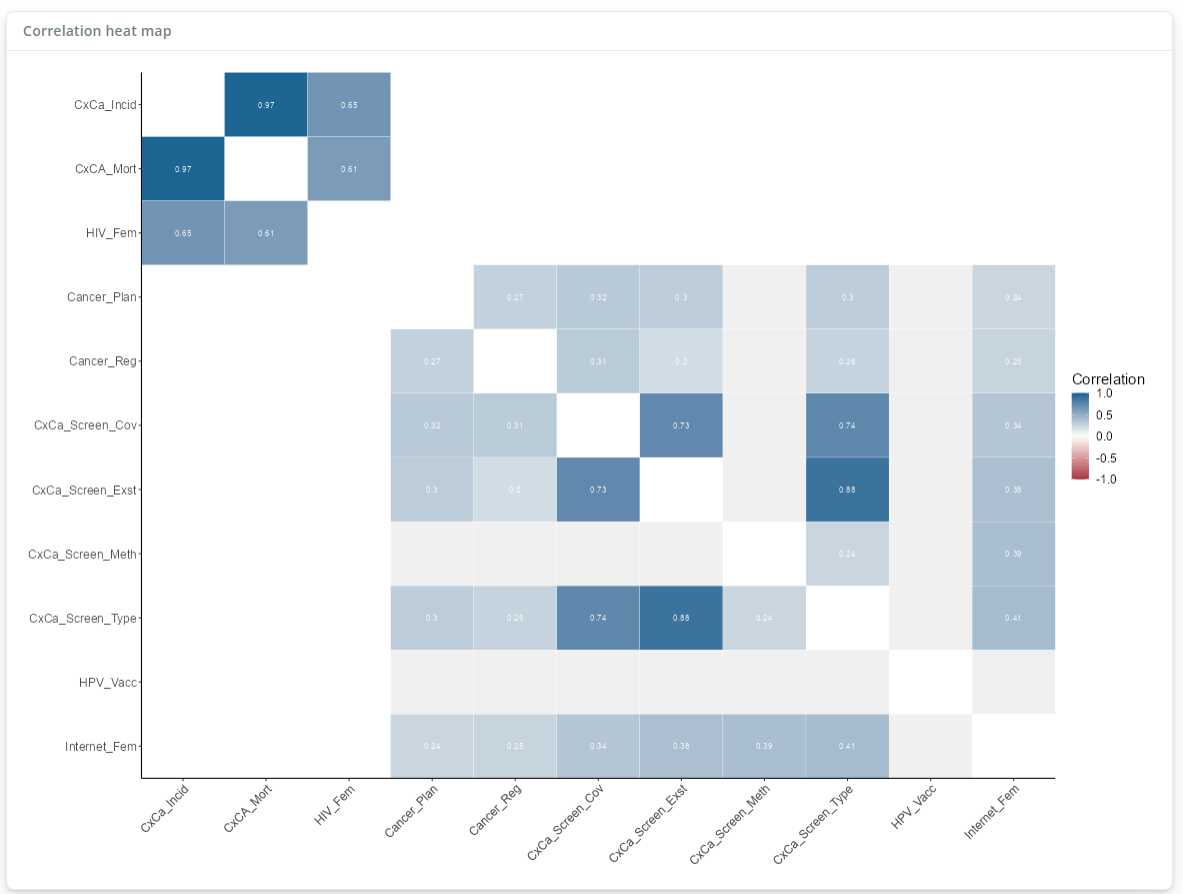
Here, we have additionally enabled the “Show values” switch, which shows the correlation values in each square, and the “Show groupings” switch (both found near the bottom of the side panel), which restricts to show only correlations between indicators within the same aggregation group.
The heatmap describes the correlation of the indicator labelled in the row, with the indicator labelled in the column, and the strength of the correlation is displayed as the colour - the colour scale is on the right. As mentioned above, what is usually of interest is very high or negative correlations, particularly between indicators within the same aggregation group.
We can select which groups to correlate against each other using the dropdown menus shown in the following figure:
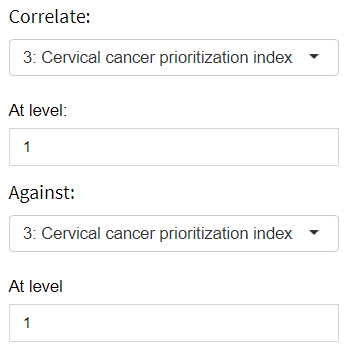
Here, the “Correlate” and “Against” dropdowns allow you to select the groups to correlate, and the “At level” dropdowns select the corresponding levels. Here, level 1 means all indicators within the selected group, but by changing to level 2, this would instead select all aggregates in level 2 within the selected group (presuming the selected group is at level 3 or higher). If this is not clear, it should be clearer after experimenting with selecting different groups and levels and seeing the results!
A useful option for quickly spotting high and negative correlations is to enable the “Discrete colours” switch. When enabled, the heat map will use a discrete (categorical) colour scale such that:
- “High” correlations (correlation above 0.9) are coloured dark green
- “OK” correlations (correlation between 0.3 - 0.9) are coloured light green
- “Weak” correlations (correlation between -0.4 - 0.3) are coloured grey
- “Negative” correlations (correlation less than -0.4) are coloured red
Although this clarifies things, please consider that these thresholds are rules of thumb and are somewhat subjective.
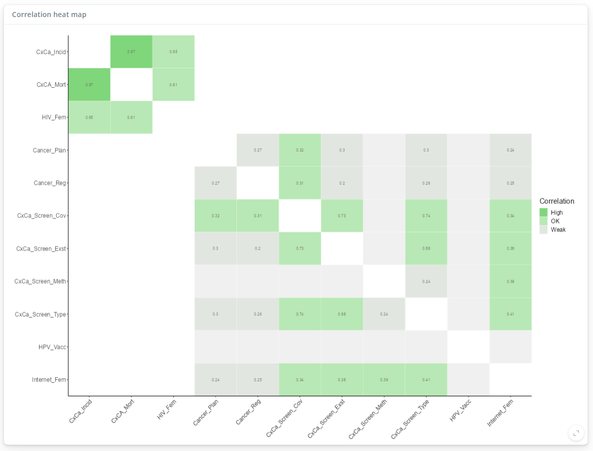
The figure above highlights two indicators that are effectively collinear (incidence rate and mortality rate) and could be reexamined.